Vector databases often look flawless in demos, then struggle once real data, real traffic, and real embeddings arrive. The core reason is simple: the search problem changes at production scale, and the trade-offs behind HNSW and IVF become much more expensive than most teams expect. At small scale, the system can hide inefficiencies; at large scale, those inefficiencies become the product. Let’s understand why vector databases fail at scale.
The 7 Performance Lies
Many teams assume a vector database that works at 1 million embeddings will behave the same at 100 million. That is usually false because scalability depends on index structure, memory layout, embedding dimensions, and query patterns, not just raw vector count.
The first lie is that “billions of vectors” automatically means good performance. In practice, the real question is latency, recall, hardware cost, and memory footprint at production scale. A system can support huge numbers on paper and still be unusable if query times are too high or infrastructure costs spiral out of control.
The second lie is that approximate nearest neighbor search behaves linearly as data grows. In reality, the curve often bends sharply after the index no longer fits comfortably in RAM. Once that happens, cache misses, memory pressure, and disk access can dominate the experience.
The third lie is that benchmarks represent real workloads. Benchmarks often use clean data, favorable hardware, and tuned parameters that hide the cost of memory thrashing, disk swapping, and tail-latency spikes. Production traffic is messier, more skewed, and more expensive to serve.
The deeper issue is that vector search is not just a software problem. It is a systems problem that combines geometry, memory, storage, and distributed coordination. That is why many databases feel fast in development but become unpredictable later.
HNSW Constant Time Lookup Myth
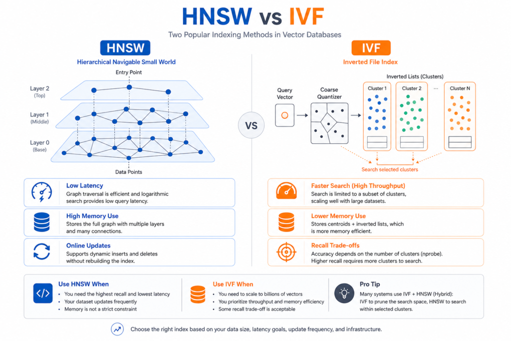
HNSW is popular because it gives fast approximate nearest neighbor search through a layered graph structure. It is designed to reduce the number of comparisons by navigating from sparse upper layers into denser lower layers, which makes it feel efficient for semantic search and RAG workloads.
The myth is that HNSW search stays close to constant time as the dataset grows. In reality, more vectors mean more graph structure, more memory overhead, and more random access, which eventually creates cache misses and slower query performance. When the graph becomes too large, the system stops behaving like an elegant graph traversal and starts behaving like a memory bottleneck.
HNSW is strong when you need online updates, good recall, and low-latency retrieval. It is especially useful when fresh embeddings keep arriving and the index must evolve without a full rebuild. That flexibility is one reason it is favored in many vector search systems.
The downside is that HNSW pays for that flexibility with memory. Each vector carries graph connections, and those connections add overhead that becomes painful at scale. Once the working set grows beyond available RAM, query performance can degrade sharply and tail latency becomes hard to predict.
A practical example makes this easier to see. At modest scale, HNSW may return near-instant results because the graph fits in memory and traversal stays cache-friendly. At much larger scale, the same traversal pattern can become random and expensive, especially when the system starts swapping or fighting for memory.
IVF Better for Scale Lie
IVF, or inverted file indexing, works by splitting the vector space into clusters and searching only the most relevant clusters at query time. This makes it attractive for large datasets because it reduces the search space and can improve throughput.
The problem is that IVF introduces a hard trade-off between speed and recall. If you search too few clusters, you miss true neighbors; if you search too many, latency rises quickly. At scale, the tuning parameter nprobe becomes a constant source of tension because it acts like a latency bandage for a deeper indexing problem.
IVF also depends heavily on the stability of the embedding distribution. If the data evolves, centroid quality degrades, clusters become imbalanced, and centroid collapse starts to reduce retrieval quality. What looked efficient on paper becomes fragile in production.
This fragility matters most when the underlying content changes over time. Product catalogs change, documents are added, topics drift, and embedding models get updated. When that happens, the cluster boundaries that once made sense may no longer represent the data well.
IVF can still be a good choice when the dataset is fairly static and the system can tolerate approximate recall. It often works well when teams can control the corpus, tune the cluster count, and monitor search quality carefully. But it is not a magic scaling solution.
Query Time Independent of Data Size Fiction
Another common misunderstanding is that vector search time is mostly independent of dataset size once indexing is in place. That is only partly true, because every index still has hidden costs tied to graph traversal, cluster probing, and candidate re-ranking.
For HNSW, deeper graphs and larger candidate pools increase the number of distance calculations. For IVF, larger datasets often require more clusters, more probes, and more expensive candidate scanning. In both cases, the system may be approximate, but it is never free.
This is why query time often rises sharply as data grows. The real cost is not only computation, but also memory access patterns, cache miss penalties, and the moment the working set no longer stays in RAM. Once the index spills into slower memory tiers or storage-backed paths, performance shifts from algorithmic to physical.
A useful way to think about it is this: the query is not only asking “Which vectors are closest?” It is also asking “How much of the index must I touch to answer that?” The more scattered the access pattern, the more expensive the query becomes.
That is why two systems with the same algorithm can perform very differently. Hardware, data distribution, and parameter choices all influence the real latency profile. A tuned setup on one dataset may collapse on another.
Embedding Dimension Impact Ignored
Vector database performance is shaped not only by the number of vectors, but also by embedding dimensions. A 1536-dimensional embedding is much more expensive to compare than a 384-dimensional one, even before you account for index overhead.
That is why dimension growth can quietly destroy performance. Higher dimensions increase memory usage, increase distance-computation cost, and make every query slower. In dense vector search, dimension count matters just as much as vector count, especially when the system already sits near the RAM limit.
This is one reason many teams run into trouble after upgrading models. A better embedding model may improve semantic quality while simultaneously increasing storage cost and lowering throughput. The result is a hidden tax on both infrastructure and latency.
The issue becomes especially visible in semantic search and RAG systems. If each query must scan or score many candidates, then every extra dimension multiplies the work. Over millions or billions of comparisons, that extra work becomes a major operational cost.
There is also a second-order effect: higher dimensions make the index itself larger. That means more memory, more pressure on caches, and a greater chance of fragmentation. Once the index starts losing locality, the system gets slower even if raw compute is still available.
Update Performance Collapse
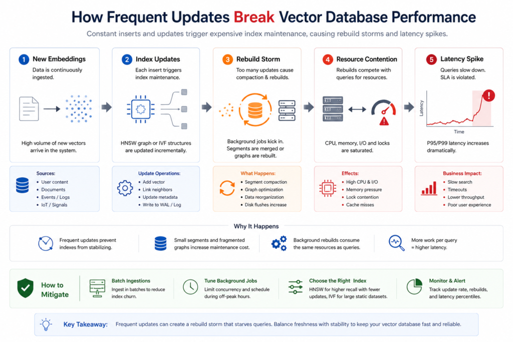
Vector databases are often sold as real-time systems, but update-heavy workloads can expose serious weaknesses. HNSW can accept inserts, yet heavy update traffic can still degrade graph quality over time. IVF can be even more fragile because cluster structure may need periodic rebuilds or retraining.
At scale, updates can trigger rebuild storms, longer ingestion times, and rising query latency. This is especially painful for RAG systems where source documents change frequently and embeddings must stay synchronized with the latest data. A system that is fast for reads can become brittle once writes increase.
The core challenge is that indexes are not passive storage structures. They are active data structures that must remain coherent as data changes. When updates arrive constantly, the index has to keep reorganizing itself, and that work competes directly with query traffic.
A practical solution is to treat updates as an architectural concern, not a background detail. Versioned embeddings, staged reindexing, and controlled rebuild windows help reduce operational risk. In many real systems, separating fresh data from stable data is more effective than trying to force one index to handle everything.
This is also why many teams adopt hybrid patterns. They may keep a hot write path for new documents and merge that path into a larger index later. That reduces operational pressure while preserving acceptable retrieval quality.
Memory Saturation Fragmentation
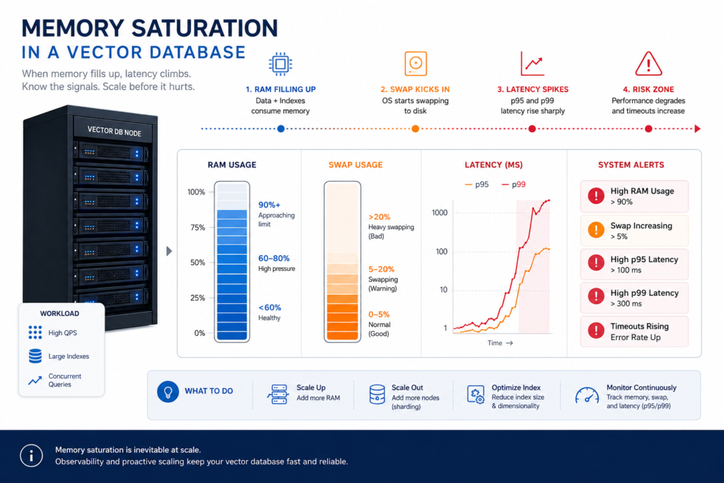
Dense vector search is fundamentally memory-hungry. HNSW stores graph connections, IVF stores cluster metadata, and both depend on fast access to large working sets. When memory pressure rises, performance often degrades long before the system fully fails.
This is where tail latency becomes dangerous. A system may still look healthy at average latency while p95 and p99 response times surge because of page faults, NUMA effects, or swapping. That makes the database feel unstable even when the core logic is still correct.
Fragmentation makes the situation worse. Even when total memory appears sufficient, the layout of allocations can prevent efficient use of available RAM. As a result, the database may still experience pauses, stalls, or uneven throughput.
For production systems, memory planning matters as much as algorithm choice. Oversizing RAM, reducing embedding dimensions, and controlling shard growth can be more valuable than another round of parameter tuning. If the index cannot stay in memory, every other optimization becomes less effective.
The lesson is simple: vector search does not fail loudly in most cases. It fails gradually, through slower tail latencies, rising variance, and operational unpredictability. That makes it easy to ignore until users begin to notice.
The Bottom Line
Vector databases fail at scale because dense search is not just an algorithm problem; it is a geometric and distributed systems problem. HNSW and IVF both help, but each introduces its own limits around memory, recall, and operational stability.
The most reliable strategy is to reduce the search space before vector search, use hierarchical or semantic sharding where appropriate, and benchmark on your own data at your own scale. If you want good recall without runaway latency, the index design must match the real workload, not the demo workload.
At production scale, the best vector database is not the one with the biggest promise. It is the one that keeps latency, memory, and retrieval quality under control when the data stops being small. That usually means designing around real constraints instead of assuming the index will scale automatically.
FAQs
1. Why do vector databases fail at scale?
Vector databases fail at scale because memory usage, query latency, embedding dimensions, and index maintenance costs grow much faster than many teams expect. HNSW and IVF both work well in smaller settings, but each can break down when the dataset becomes too large or the workload changes.
2. What is the difference between HNSW and IVF indexing?
HNSW uses a layered graph to navigate toward nearest neighbors quickly, while IVF splits vectors into clusters and searches only the most relevant clusters. HNSW usually offers better recall and online updates, while IVF can be cheaper for large static datasets if tuned well.
3. Which is better for large-scale vector search: HNSW or IVF?
Neither is universally better. HNSW is often stronger for low-latency semantic search and frequent updates, while IVF can scale well for static or mostly stable data if you can manage the recall-latency trade-off.
4. Why does HNSW slow down as data grows?
HNSW slows down because the graph becomes larger, memory overhead increases, and random access patterns create more cache misses. Once the index no longer fits comfortably in RAM, latency can rise sharply.
5. Why does IVF lose recall at scale?
IVF loses recall because it only searches a limited number of clusters. If the nearest neighbors fall outside the selected clusters, the system misses relevant results unless you increase the number of probes, which also increases latency.
6. How do embedding dimensions affect vector database performance?
Higher embedding dimensions increase storage size and distance-computation cost. A model with 1536 dimensions will usually require more memory and more processing than one with 384 or 768 dimensions.
7. What is centroid collapse in IVF?
Centroid collapse happens when some clusters become overloaded while others remain underused. This imbalance reduces retrieval quality and often forces teams to increase search probes just to maintain acceptable recall.
8. How can I improve vector database performance at scale?
You can improve performance by reducing embedding dimensions, pre-filtering data before vector search, using semantic or hierarchical sharding, and tuning HNSW or IVF parameters for your actual workload. Benchmarking on your real data is essential.
9. Are vector databases good for real-time updates?
Some are, but update-heavy workloads are difficult at scale. HNSW handles incremental inserts better than IVF, but both can suffer when updates are frequent, large, or poorly managed.
10. What is the biggest mistake teams make with vector databases?
The biggest mistake is trusting small-scale benchmarks. Results at 1 million vectors often do not predict behavior at 100 million vectors, especially when RAM usage, embedding size, and operational overhead are ignored.